α-Stable Distribution and its Applications in Cellular Networks

Introduction

Enabled by wireless Big Data, this website is proudly reserved for $\alpha$-Stable distribution and its applications in wireless cellular networks, the works of which have been recently completed by Rongpeng Li, Yifan Zhou, Meng Li, Chen Qi, Xuan Zhou, Zhifeng Zhao and Honggang Zhang from Zhejiang University, Hangzhou, China, and Luca Chiaraviglio, Francesca Cuomo, Andrea Gigli, Maurizio Maisto from University of Rome, Sapienza, Rome, Italy, respectively.

Based on practical Big Data measurements of on-operating cellular networks, they unveiled the suitability of $\alpha$-Stable distribution in several scenarios of cellular networks, including spatial distribution of base station, dependence between  base stations deployment and traffic spatial distribution,  temporal distribution of traffic series. Meanwhile, several interesting features could be well explained by $\alpha$-Stable distributions. In particular, rooted in the $\alpha$-Stable distribution, it has been found that fractal patterns, scale-free law and Small-World features coexist in the complex wireless “cellular” networks.

MATLAB source codes:

1. The MATLAB source codes for base station spatial distribution identification can be downloaded here:  BS_density_pdf.

Model Description

Following the generalized central limit theorem, $\alpha$-Stable models manifest themselves in the capability to approximate the distribution of normalized sums of a relatively large number of independent identically distributed random variables. Besides, $\alpha$-Stable models produce strong bursty results with properties of heavy-tailed distributions and long range dependence [1]. Therefore, they arose in a natural way to characterize the traffic in fixed broadband networks [2,5] and have been exploited in resource management analyses [8,9].

$\alpha$-Stable models, with few exceptions, lack a closed-form expression of the PDF, and are generally specified by their characteristic functions.

Definition

A random variable $X$ is said to obey $\alpha$-Stable models if there are parameters $0<\alpha \le 2$, $c\ge 0$, $-1\le \beta \le 1$, and $\mu \in \mathcal{R}$ such that its characteristic function is of the following form:

• If $\alpha =1$, $\mathrm{\Phi }(\omega )=E(\exp j\omega X)=\exp -\sigma |c|(1+j\beta (\text{sgn}(c))\ln |c|)+j\mu c$;
• Otherwise, $\mathrm{\Phi }(\omega )=E(\exp j\omega X)=\exp -{\sigma }^{\alpha }|c{|}^{\alpha }(1-j\beta (\text{sgn}(c))\tan \frac{\pi \alpha }{2})+j\mu c$.

Here, the function $E(\cdot )$ represents the expectation operation with respect to a random variable. $\alpha$ is called the characteristic exponent and indicates the index of stability, while $\beta$ is identified as the skewness parameter. $\alpha$ and $\beta$ together determine the shape of the models. Moreover, $c$ and $\mu$ are called scale and shift parameters, respectively. Specifically, if $\alpha =2$, $\alpha$-Stable models reduce to Gaussian distributions.

Furthermore, for an $\alpha$-Stable modeled random variable $X$, there exists a linear relationship between the parameter $\alpha$ and the function $\mathrm{\Psi }(\omega )=\ln -\text{Re}\ln (\mathrm{\Phi }(\omega ))$ as $\mathrm{\Psi }(\omega )=\ln -\text{Re}\ln (\mathrm{\Phi }(\omega ))=\alpha \ln (\omega )+\alpha \ln (\sigma ),$ where the function $\text{Re}(\cdot )$ calculates the real part of the input variable.

Figure Illustrations

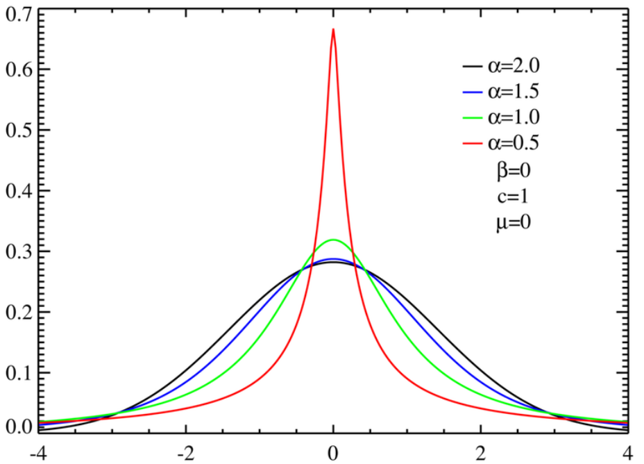
Symmetric $\alpha$-Stable distributions with unit scale factor. Courtesy to Wikipedia.

Skewed centered Stable distributions with unit scale factor. Courtesy to Wikipedia.

Validation Methodology

Usually, it’s challenging to prove whether a dataset follows a specific distribution, especially for $\alpha$-Stable models without a closed-form expression for their PDF. Therefore, when a dataset is said to satisfy $\alpha$-Stable models, it usually means the dataset is consistent with the hypothetical distribution and the corresponding properties. In other words, the validation needs to firstly estimate parameters of $\alpha$-Stable models from the given dataset, and then compare the real distribution of the dataset with the estimated $\alpha$-Stable model. Specifically, the corresponding parameters in $\alpha$-Stable models can be determined by quantile methods, or sample characteristic function methods.

Useful references

1. G. Samorodnitsky, Stable Non-Gaussian Random Processes: Stochastic Models with Infinite Variance. New York: Chapman and Hall/CRC, 1994.
2. J. R. Gallardo, D. Makrakis, and L. Orozco-Barbosa, “Use of alpha-Stable self-similar stochastic processes for modeling traffic in broadband networks,” in Proc. SPIE Conf. P. Soc. Photo-Opt. Ins, Boston. Massachusetts, Nov. 1998, vol. 3530, pp. 281–296.
3. S. M. Koyon and D. B. Williams, “On the characterization of impulsive noise with $\alpha$-Stable distributions using Fourier techniques,” in Proc. Asilomar Conf. Signals, Systems, Computers, Oct. 1995.
4. J. B. Hill, “Minimum Dispersion and Unbiasedness: ‘Best’ Linear Predictors for Stationary ARMA a-Stable Processes,” University of Colorado at Boulder, Discussion Papers in Economics Working Paper No. 00-06, Sep. 2000.
5. X. Ge, G. Zhu, and Y. Zhu, “On the testing for alpha-Stable distributions of network traffic,” Comput. Commun., vol. 27, no. 5, pp. 447–457, Mar. 2004.
6. A. Karasaridis and D. Hatzinakos, “Network heavy traffic modeling using alpha-Stable self-similar processes,” IEEE Trans. Commun., vol. 49, no. 7, pp. 1203–1214, Jul. 2001.
7. P. Zagaglia, “Estimation of alpha-Stable distribution parameters using a quantile method,” 25-Jan-2012. [Online]. Available: http://www.mathworks.com/matlabcentral/fileexchange/34783-estimation-of-alpha-Stable-distribution-parameters-using-a-quantile-method. [Accessed: 09-Oct-2014].
8. W. Song and W. Zhuang, “Resource Reservation for Self-Similar Data Traffic in Cellular/WLAN Integrated Mobile Hotspots,” in Proc. IEEE ICC 2010, Cape Town, South Africa, May 2010.
9. J. C.-I. Chuang and N. R. Sollenberger, “Spectrum resource allocation for wireless packet access with application to advanced cellular Internet service,” IEEE J. Sel. Area. Comm., vol. 16, no. 6, pp. 820–829, Aug. 1998.
10. Rongpeng Li, Zhifeng Zhao, Chen Qi, Xuan Zhou, Yifan Zhou, and Honggang Zhang, “Understanding the Traffic Nature of Mobile Instantaneous Messaging in Cellular Networks: A Revisiting to alpha-Stable Models” , IEEE Access, vol. 3, pp. 1416-1422, 2015.
11. Luca Chiaraviglio, Francesca Cuomo, Maurizio Maisto, Andrea Gigli, Josip Lorincz, Yifan Zhou, Zhifeng Zhao, Chen Qi, Honggang Zhang, “What is the Best Spatial Distribution to Model Base Station Density? A Deep Dive in Two European Mobile Networks”, IEEE Access, Apr. 2016.
12. Yifan Zhou, Rongpeng Li, Zhifeng Zhao, Xuan Zhou, and Honggang Zhang, “On the $\alpha$-Stable Distribution of Base Stations in Cellular Networks”, IEEE Communications Letters, vol. 19, no. 10, pp. 1750-1753, Aug. 2015.

Spatial Distribution of Base Stations

Motivation

Confronting the fundamental challenges of the long-term evolution of the ever-growing complication, heterogeneity and densification in wireless cellular networks (2G/3G/LTE/5G), the networking architecture and the base stations spatial distribution have been expressing the features of geometric topology irregularity.

Basically, in the wireless cellular networks, the base stations (BSs) appear to be the essential part in the whole system.  The spatial structure of BSs has a great impact on the performance of cellular networks, since the received signal strength varies depending on the distance between transmitter and receiver. Moreover, interference characterization is very complicated and challenging due to path loss and multipath fading effect, in particular for a heterogeneous networking (HetNets) scenario consisting of different types of BSs. In order to evaluate the network performance more accurately and tractably, it is essential to obtain realistic spatial models for the BSs deployment in cellular networks.

Recently, Poisson distribution has been widely adopted to characterize the spatial distribution of BSs, and leads to a tractable approach to calculate the coverage probability and rate distribution in cellular networks, by taking advantage of a Poisson point process (PPP) based theory (i.e., stochastic geometry). However, the modeling accuracy of Poisson distribution has been recently questioned in regard to a number of realistic cellular networking scenarios. Consequently, in order to reduce the modeling error between Poisson distributed BSs and the practical distributed ones, some variants of PPP have been exploited to obtain precise analysis results. On the other hand, the actual deployment of BSs in long term is highly correlated with human activities.

Inspired by the clustering reality of BSs and the intrinsic heavy-tailed characteristics of human activities, we aim to re-examine the statistical pattern of BSs in cellular networks, and find the most appropriate spatial density distribution of BSs. Interestingly, by taking advantage of large amount (Big Data) of realistic deployment information of BSs from on-operating cellular networks around the world, we find that the widely adopted Poisson distribution (i.e. PPP) severely diverges from the practical/actual spatial distribution of BSs. Instead, heavy-tailed distributions could more precisely match the practical/actual distribution. In particular, $\alpha$-S****table distribution, the heavy-tailed distribution also found in various traffic patterns of wired broadband networks and wireless cellular networks, is most consistent with the practical/actual measured data. Moreover, rooted in the $\alpha$-Stable distribution, it has also been found that fractal patterns, scale-free law and Small-World features coexist in the complex wireless “cellular” networks.

Moreover, by in-depth statistical comparisons based on the above large-scale (Big Data) identification, we also investigated the Gibbs point processes (Geyer, Strauss & PHCP) as well as the Neyman-Scott point processes (MCP & TCP: Matern cluster process & Thomas cluster process),  and compared their performance in the view of a large-scale modeling test, and finally found the general clustering nature of BSs deployment. However, either Gibbs point processes (Geyer, Strauss & PHCP) or Neyman-Scott point processes (MCP & TCP), diverged from the practical/actual spatial distribution of BSs, to some extent (see the following Table).

In summary, we have carried out an large-scale identification based on real data of base station locations from both Chinese and European mobile operators. For detailed description, please check the subsections on this topic as well as the following references.

---

Related references:

• Yifan Zhou, Rongpeng Li, Zhifeng Zhao, Xuan Zhou, and Honggang Zhang, “On the $\alpha$-Stable Distribution of Base Stations in Cellular Networks“, IEEE Communications Letters, vol. 19, no. 10, pp. 1750-1753, Aug. 2015.

• Rongpeng Li, Zhifeng Zhao, Yi Zhong, Chen Qi, and Honggang Zhang, “The Stochastic Geometry Analyses of Cellular Networks with $\alpha$-Stable Self-Similarity,” IEEE Trans. on Communications, March 2019.

• Ying Chen, Rongpeng Li, Zhifeng Zhao, and Honggang Zhang, “Study on Base Station Topology in National Cellular Networks: Take Advantage of Alpha Shapes, Betti Numbers, and Euler Characteristics,” IEEE Systems Journal, Q3/Q4 2019

• Ying Chen, Rongpeng Li, Zhifeng Zhao, and Honggang Zhang, “Fundamentals on Base Stations in Urban Cellular Networks: From the Perspective of Algebraic Topology,” IEEE Wireless Communications Letters, April 2019.

• Yifan Zhou, Zhifeng Zhao, Yves Louet, Qianlan Ying, Rongpeng Li, Xuan Zhou, Xianfu Chen, and Honggang Zhang, “Large-scale Spatial Distribution Identification of Base Stations in Cellular Networks,”  IEEE Access, vol. 3, pp. 2987-2999, Dec. 2015. 

• Zhifeng Zhao, Meng  Li, Rongpeng Li, and Yifan Zhou, “Temporal-Spatial Distribution Nature of Traffic and Base Stations in Cellular Networks,” IET Communications, Q3 2017.

• Luca Chiaraviglio, Francesca Cuomo, Maurizio Maisto, Andrea Gigli, Josip Lorincz, Yifan Zhou, Zhifeng Zhao, Chen Qi, Honggang Zhang, “What is the Best Spatial Distribution to Model Base Station Density? A Deep Dive in Two European Mobile Networks,” IEEE Access, Apr. 2016.

• Luca Chiaraviglio, Francesca Cuomo, Andrea Gigli, Maurizio Maisto, Yifan Zhou, Zhifeng Zhao, Honggang Zhang, “A Reality Check of Base Station Spatial Distribution in Mobile Networks,” IEEE INFOCOM 2016 (Poster), San Francisco, Apr. 2016.

China Datasets

Background

Data description

In order to reach credible results, we collect a massive amount of practical data of BSs information from China Mobile in a well-developed eastern province of China. The collected dataset, containing over 47,000 BSs of GSM cellular networks and serving  over 40 million subscribers, encompasses all BS-related records like location information (i.e. longitude, latitude, etc.) and BS type (i.e. macrocell or microcell). Based on the coverage area and location information, we divide the dataset into disjoint subsets. Accordingly, we can classify the data set as subsets of urban areas and rural areas, by matching the geographical land forms with local maps, as depicted in Fig. 1.

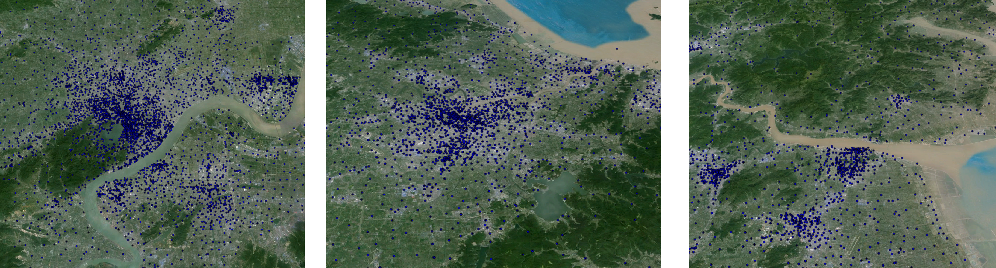
Fig. 1 An illustration of the deployment of base stations in three typical cities with geographical landforms, namely City A, B, C, respectively.

Mathematical model

Heavy-tailed distributions could be widely applied to explain a number of natural phenomena, including the Internet topology. Mathematically, heavy-tailed distributions are probability distributions whose tails are not exponentially bounded. In other words, they have heavier tails than the exponential distribution.

There exist many statistical distributions proving to be heavy-tailed. Among them, generalized Pareto (GP) distribution, Weibull distribution, and log-normal distribution belong to one-tailed ones with the probability density function (PDF) in closed-forms (see Table II). Another famous heavy-tailed distribution is $\alpha$-Stable distribution, who manifests itself in the capability to characterize the distribution of normalized sums of a relatively large number of independent identically distributed random variables. However, $\alpha$-Stable distribution, with few exceptions, lacks a closed-form expression of the PDF, and is generally specified by its characteristic function, as presented in the model description page.

TABLE II: The List of Candidate Distributions and Estimated Parameters.

Statistical Pattern of Base Stations with Large-scale Identification

 Based on the large amount of BS location data, we sample one certain city randomly with a fixed sample area size. Then, we compute the spatial density for different 10000 sample areas and obtain the empirical density distribution, by counting and sorting the number of BSs in each sample area. Next, we estimated the unknown parameters in candidate distributions (except $\alpha$-Stable distribution) using maximum likelihood estimation (MLE) methodology. For $\alpha$-Stable distribution, we estimate the relevant parameters using quantile methods, correspondingly build the model to generate the corresponding random variable, and finally compare its induced PDF with the exact (empirical) one.

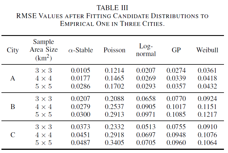
 In the first place, we refer to City B as an example, and compute the PDF of BS density under the sample area size 4×4 km ² . After fitting the corresponding PDF to distributions in Table II, we provide the comparison between the empirical BS density distribution with candidate ones in Fig. 2 and Fig. 3. As depicted in Fig. 3, the statistical pattern of BSs obviously exhibits heavy-tailed characteristics. Besides, among all candidate distributions, $\alpha$ -Stable distribution most precisely match the empirical PDF. On the other hand, we provide the numerical comparison in Table III, in terms of root mean square error (RMSE). Indeed, the RMSE results in Table III show $\alpha$-Stable distribution has the minimum RMSE value (0.0279) while Poisson distribution has the maximum one (0.2537), and once again strengthen this aforementioned conclusion. All of the estimated parameters of the fitted candidate distributions are also listed in Table II.

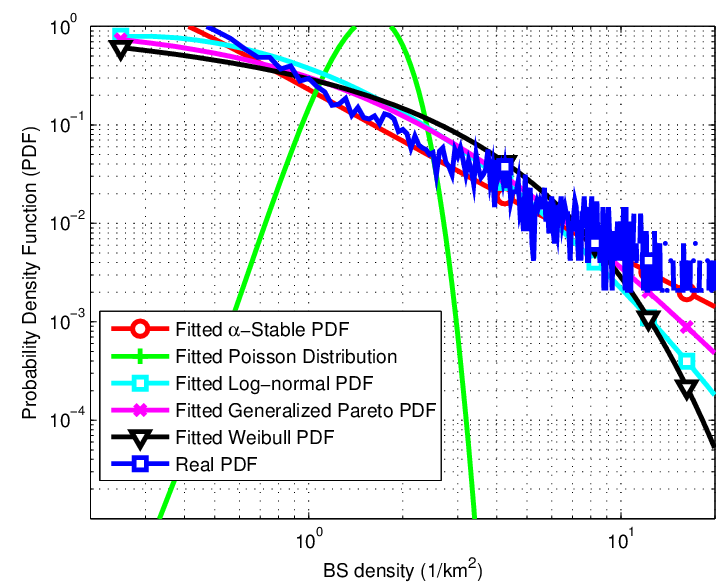
Fig. 2: The log-log comparison between practical BS density distribution in City B with candidate ones, when sample area size equals 4×4 km².

5×5 km².

In order to examine the geographical impact on the fitting results, we further analyze the density distribution of BSs in City A and City C using a sample area size of 4×4 km². Due to the factor of geographical irregularity, there is a noticeable gap between the $\alpha$-Stable distribution and the empirical PDF of City A and C in comparison with City B. Nevertheless, as shown in Table III and Fig. 4, it can be observed that, $\alpha$-Stable distribution could match the practical one in both cities, with RMSE values equaling 0.0177 and 0.0451 respectively and being less than those of other candidate distributions. Moreover, the same conclusions concerned with sample area sizes of 3×3 km ² and 5×5 km ², could be also testified in Table III.

Based on the extensive analyses above, we could confidently reach the following remark.

The spatial pattern of deployed BSs exhibits strong heavy-tailed characteristics. Based on the large-scale identification, $\alpha$-Stable distribution manifests itself as the most precise one. On the contrary, the popular Poisson distribution is an inappropriate model for the BS density distribution, in terms of the root mean square error.

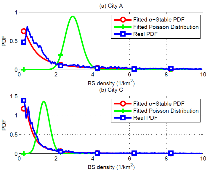
Fig. 4. The comparison between BS density distribution and $\alpha$-Stable distribution in City A and City C, when sample area size equals 4×4 km².

Conclusions and Future Works

Based on the practical BS deployment information of one on-operating cellular networks, we carried out a thorough investigation over the statistical pattern of BS density. Our study showed that the distribution of BS density exhibits strong heavy-tailed characteristics. Furthermore, we found that the widely adopted Poisson distribution severely diverges from the realistic distribution. Instead, $\alpha$-Stable distribution, the distribution also found in the traffic dynamics of broadband networks and cellular networks, most precisely match the practical one. Moreover, our study could contribute to the understanding of evolution trend of BS deployment, as well as the impact of human social activities in long term.

Currently, the lack of closed-form for $\alpha$-Stable distribution makes it difficult to reach tractable solutions and might hinder its applications in networking performance (e.g., coverage, rate, etc) analyses. Therefore, we are dedicated to handle the related meaningful yet more challenging issues over applications of $\alpha$-Stable distribution in the future.

Related references:

•  Yifan Zhou, Rongpeng Li, Zhifeng Zhao, Xuan Zhou, and Honggang Zhang, “On the $\alpha$-Stable Distribution of Base Stations in Cellular Networks“, IEEE Communications Letters, vol. 19, no. 10, pp. 1750-1753, Aug. 2015. 

• Yifan Zhou, Zhifeng Zhao, Yves Louet, Qianlan Ying, Rongpeng Li, Xuan Zhou, Xianfu Chen, and Honggang Zhang, “Large-scale Spatial Distribution Identification of Base Stations in Cellular Networks,”  IEEE Access, vol. 3, pp. 2987-2999, Dec. 2015. 

• Zhifeng Zhao, Meng  Li, Rongpeng Li, and Yifan Zhou, “Temporal-Spatial Distribution Nature of Traffic and Base Stations in Cellular Networks,” IET Communications, August 2017.

• Rongpeng Li, Zhifeng Zhao, Yi Zhong, Chen Qi, and Honggang Zhang, “The Stochastic Geometry Analyses of Cellular Networks with alpha-Stable Self-Similarity,” arxiv.org/abs/1709.05733v1, September 2017.

European Datasets

Data Description

Itallian dataset description

We initially focus on the Emilia-Romagna region of Italy, which is covered by four different cellular operators (referred as A, B, C and D in the following). Table 1 reports the main features of the considered dataset. The total number of deployed BSs considering the whole set of operators is more than 4900 BSs. Focusing then on each operator, the number of deployed BSs is similar for operator A and operator B, while it is slightly lower for operators C and D. More in depth, operator D reuses part of the cellular infrastructure of the two largest operators to guarantee coverage in the zones not covered by its own BSs. As for the morphological characteristics of the area, the whole region spans over 22000 km^2^, which includes rural areas, town areas and one metropolitan area. This is also reflected in the number of subscribers, which is larger than 6.5 millions in total, with the largest number of subscribers living in the metropolitan area. Finally, the average BS density (i.e., the total number of deployed BSs for each operator over the total region), is always lower than one, due to the fact that in rural areas less BSs are deployed compared to urban ones. However, the density is larger for operator A and B, and slightly lower for the other operators.

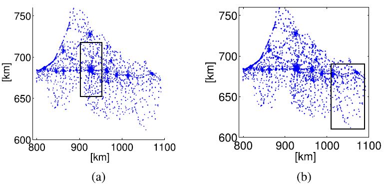
FIGURE 1. Italian Dataset: BS positions and considered scenarios (inside the rectangular boxes). (a) IT urban scenario. (b) IT rural scenario.

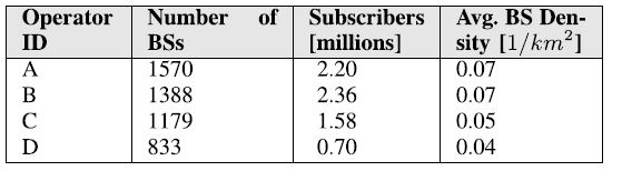
TABLE 1. Main features of the Italian data set.

CROATIAN dataset description

In addition to the Italian dataset, we have considered the set of BSs sites having freestanding masts from the country of Croatia. In particular, more than 2600 BSs are deployed in an area of around 56000 km^2^. The database is composed of the BSs sites owned by the telecom operators currently active in Croatia, serving in total more than 4.6 millions of users. The morphological characteristics of the country include one large metropolitan area around the capital Zagreb, different rural zones, and one coastal zone including most of tourist attractions. In addition to the BSs sites actually deployed in the network, the positions of planned BSs sites to be installed in the future is also provided, considering a vast region in the north of the country. Moreover, Table 2 reports the characteristics of each scenario in terms of: number of considered BSs, size of the area, and average BS density.

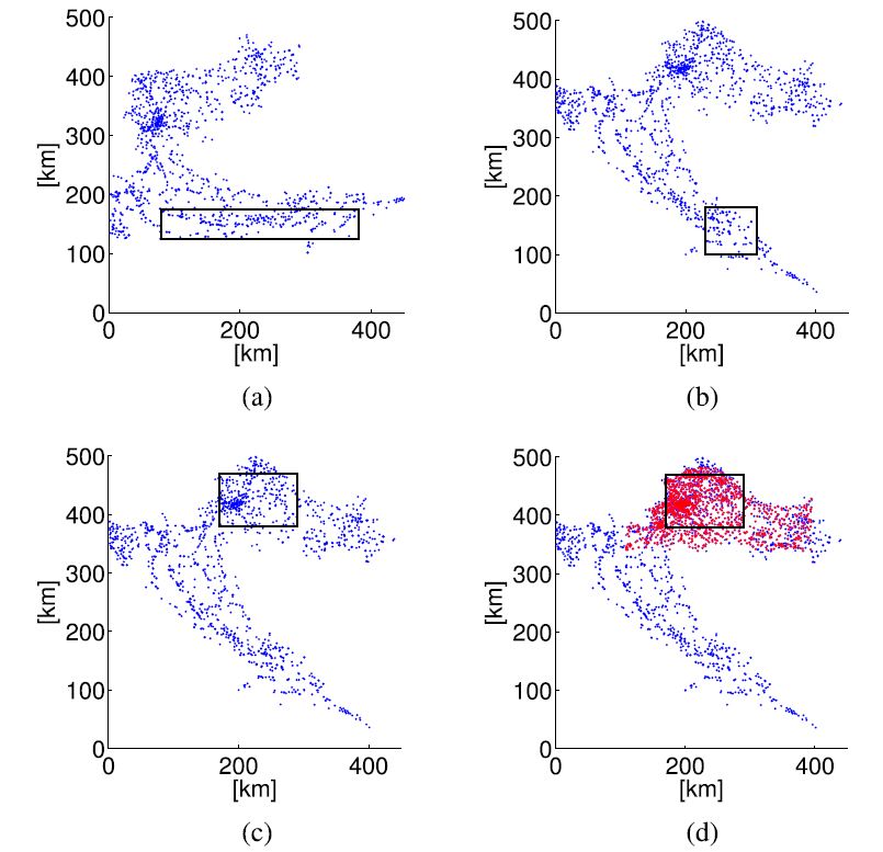
FIGURE 2. Croatian Dataset: BS positions and considered scenarios (inside the rectangular boxes). (a) CRO coastal scenario. (b) CRO rural scenario. (c) CRO urban scenario. (d) CRO urban scenario including future planned BSs.

Model Description

The mathematical models adopted here are the same with that in China dataset.

Case-Studies Results

Given the BS positions in each scenario, we then compute the empirical spatial distribution of the BS density. Initially, we sample each scenario with a small area of fixed size. We then randomly select 10000 squares of fixed area size. For each square, we compute the number of BSs falling into it. This number, divided by the area size, represents the BS density. From the BS densities, we derive the PDF. This spatial distribution is then used as reference one vs. the possible candidates (i.e., Poisson, GP, Weibull, Lognormal and $\alpha$-Stable). For each candidate distribution, we estimate the unknown parameters by applying the Maximum Likelihood Estimation (MLE) criterion. For estimating the parameters of the $\alpha$-Stable distribution, we adopted a similar procedure like the one reported in, due to the fact that the closed-form for this distribution does not always exist.

We initially focus on the urban area of the Italian scenario. As a showcase, we compute the PDF of BS density with a sample area of size 10 x10 km^2^. Moreover, we have taken into account the BSs from all the operators in order to maximize the number of BSs under consideration. Fig. 3 reports the empirical PDF (i.e., the real one) with the fitting of various candidate distributions. Interestingly, the best fitting is obtained with the $\alpha$-Stable distribution, while the other ones perform consistently worse.

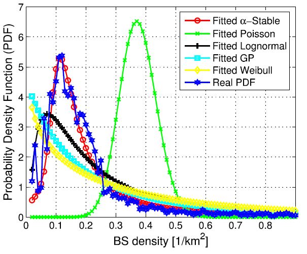
FIGURE 3. Italian urban scenario: probability density function of the BS density with all operators and sample squared area with size 100 km^2^.

In the following, we have computed the Root Mean Square Error (RMSE) of the different fittings against the empirical PDF. This metric is useful to capture the fitting accuracy of the considered distribution. In this case, for modeling generalization purpose, we have also considered the variation of the sample area between 5x5 km^2^ and 11x11 km^2^ in the scenario. Recall that for each sample area size we randomly select 10000 samples in the scenario. Fig. 4 illustrates the obtained results. Obviously, the $\alpha$-Stable is the best fitting for all the considered sample areas, with a RMSE always lower than 0.3. On the other hand, the Poisson distribution exhibits a RMSE always larger than 0.5, thus confirming our intuition that it is not suitable to capture the spatial density distribution of real BSs.

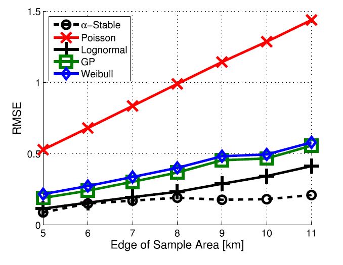
FIGURE 4. Italian urban scenario: RMSE vs. size of the sample squared area.

Furthermore, we have investigated the impact of single operators. Fig. 5(a) reports the RMSE values for each single operator. Recall that A and B exhibit the largest number of BSs, while operator D tends to exploit the BSs of the other operators to provide user coverage. Surely, the $\alpha$-Stable is the best fitting for operators A, B and C. On the contrary, for operator D the $\alpha$-Stable RMSE is lower than the Poisson distribution but higher than the other ones. This is due to the fact that this operator does not spread its own BSs in the same way like the other ones, resulting in a different density distribution. Moreover, we can see that the RMSE tends to increase from left to right (i.e., towards operators with less BSs). To give more insight, Fig. 5(b) provides the results when multiple operators are considered to compute the BS density.

FIGURE 5. Italian urban scenario: RMSE for single and multiple operators. (a) Single operators. (b) Multiple operators.

Interestingly, the $\alpha$-Stable fitting tends to be almost constant, while the RMSEs of the other distributions tend to increase when the number of operators is decreased. In particular, operator A, which is also the largest one, has deployed its BSs in the scenario in order to always provide coverage to users with its own BSs. On the contrary, operator D tends to lease the infrastructure from the other operators. The case with the single operator A matches better a complete BSs deployment in the targeted region, resulting in a low RMSE with the $\alpha$-Stable model.

TABLE 2. Italian urban scenario: RMSE values vs. BS technology.

In the following part we have taken into account the impact of various cellular networking technologies on the BS density. Together with each BS position, in fact, our dataset includes information about the technology, which can be GSM, UMTS, LTE, or not specied. Each BS entry in the BS database includes a list of the supported technologies. Specifically, by manually checking in the BS database, we have found that the UMTS service is always provided in the considered region, except for the BSs for which the technology is not specied. At the same time, when the LTE service is provided, also GSM and UMTS services are available. Therefore, we have considered the following categories: GSM/UMTS, GSM/UMTS/LTE, or the entire dataset (i.e., including the BSs for which the technology is not specified). For each category, we have then computed the empirical PDF as well as the distribution fitting. Table 2 describes the obtained RMSE values. Once again, these results confirm that the $\alpha$-Stable fitting reaches the highest accuracy in this scenario, while all the other distributions have a RMSE at least more than doubled.

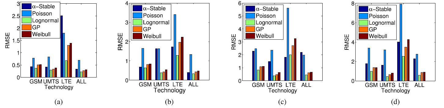
FIGURE 6. Italian rural scenario results. (a) Sample area size 5x5 km^2^. (b) Sample area size 7x7 km^2^. (c) Sample area size 9x9 km^2^. (d) Sample area size 11x11 km^2^.

In the following, we have moved our attention to the Italian rural scenario. Differently, from the previous case, in this scenario there are no big towns, and the BS distribution over the territory is rather sparse. In order to evaluate the behavior of the different distributions, we have computed the RMSE for different sample area sizes, and for different technologies, as reported in Fig. 6. As expected, the Poisson distribution does not adhere to the empirical distribution, resulting in the highest RMSE. The other distributions tend to have a lower RMSE. Among them, the best candidate is the Lognormal distribution in most of the cases. On the contrary, the $\alpha$-Stable distribution exhibits a higher RMSE than the Lognormal one (but lower than the Poisson one). This fact is confirmed across the different technologies, and for the different area sizes. Therefore, the $\alpha$-Stable distribution is useful to capture the BS spatial behavior in urban maps. When the BS distribution becomes more sparse than in a city, like in this case, the best candidates are other types of distributions (i.e., like the Lognormal one in this case).

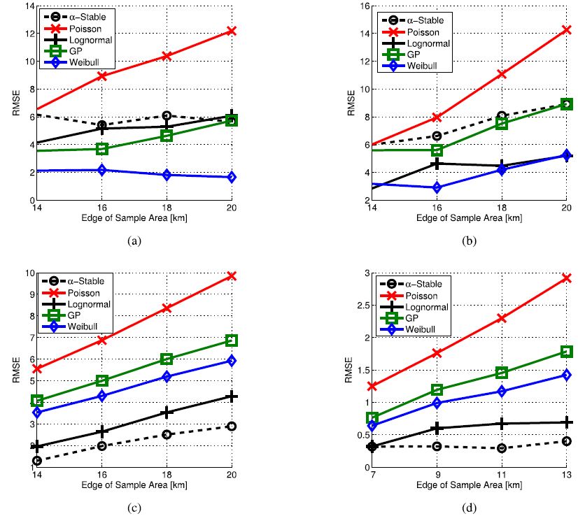
FIGURE 7. Croatian scenarios: RMSE of the distributions for different sample area sizes. (a) Coastal. (b) Rural. (c) Urban. (d) Urban with Future Planned BSs.

We have investigated in the next step the Croatian scenarios. Fig. 7 reports the obtained results in terms of RMSE for the different distributions. In this case, we have also varied the size of the sample area. Particularly, since the BSs are rather sparse in the rural, coastal and urban scenarios (without planned BSs), we have adopted a larger sample area size than the Italian cases (i.e., ranging between 14x 14 km^2^ and 20x20 km^2^). On the contrary, we have adopted a sample area comparable with the Italian case for the urban scenario with future planned BS, since the BS density is quite similar in these two cases. Focusing on the obtained results, the best fitting for the coastal case is the Weibull distribution (reported in Fig. 7(a)), while the Lognormal one tends to achieve comparable RMSE values when the rural case in considered (see Fig. 7(b)). However, when the urban scenarios are considered (Fig. 7(c) and Fig. 7(d)) the distribution achieving the lowest RMSE is the $\alpha$-Stable. This fact further confirms our intuition that the $\alpha$-Stable model matches the BS spatial distribution in urban areas. Moreover, our results also imply that the definition of a universal model, covering all kinds of urban, coastal, and rural scenarios, is still an open issue.

Conclusions and Future Works

We have studied the BS spatial distributions across different scenarios obtained from Italy and Croatia, considering urban, coastal, and rural zones.We have compared the real distribution against different candidate ones. Our results show that the best distribution matching the real one is the $\alpha$-Stable model in urban scenarios. This fact is confirmed across different sample area sizes, operators, and technologies. On the contrary, the Lognormal and Weibull distributions tend to fit better the real one in coastal and rural scenarios. We believe that this work can be used to derive fruitful guidelines for the BS deployment. As next step, we will complement these findings with a detailed study of spatial and temporal variations of user traffic. Moreover, we will extend our analysis to other countries (such as in Asia and in North America). Finally, we will study the possibility of deriving a universal model covering rural, urban and coastal zones.

Related references:

• Luca Chiaraviglio, Francesca Cuomo, Maurizio Maisto, Andrea Gigli, Josip Lorincz, Yifan Zhou, Zhifeng Zhao, Chen Qi, Honggang Zhang, “What is the Best Spatial Distribution to Model Base Station Density? A Deep Dive in Two European Mobile Networks,” IEEE Access, Apr. 2016. 

• Luca Chiaraviglio, Francesca Cuomo, Andrea Gigli, Maurizio Maisto, Yifan Zhou, Zhifeng Zhao, Honggang Zhang, “A Reality Check of Base Station Spatial Distribution in Mobile Networks,” IEEE INFOCOM 2016 (Poster), San Francisco, Apr. 2016.

• Rongpeng Li, Zhifeng Zhao, Yi Zhong, Chen Qi, and Honggang Zhang, “The Stochastic Geometry Analyses of Cellular Networks with alpha-Stable Self-Similarity,” arxiv.org/abs/1709.05733v1, September 2017.

Temporal Distribution of Traffic Series (Mobile Traffic Big Data)

Background

Mobile instant messaging (MIM) services significantly facilitate personal and business communications, inevitably consume substantial network resources, and potentially affect the network stability. It is meaningful to carefully examine the traffic nature of MIM (e.g. WeChat/Weixin) services, so as to design MIM service-oriented protocols to overcome their induced negative influence to cellular networks.

MIM Working Mechanisms

MIM services, which solely rely on mobile Internet to exchange information, have quite working mechanisms from traditional short messaging services. One of the prominent differences is that born with stanard protocols, traditional short messaging services could conveniently fulfill timely information delivery and provision “always-online” service. However, for mobile Internet in packet switching domain, a TCP connection would release itself if exceeding a TCP inactivity timer. Therefore, as depicted in the above picture, besides transmitting (TX) and receiving (RX) normal packets after logging onto a server, MIM services commonly take advantages of keep-alive mechanisms to send packets containing little information periodically and maintain a long-lived TCP connection.

Hereinafter, message refers to a series of packets transmitted between the user equipment (UE) and the servers of service provider on application layer. Therefore, the messages delivered on every TCP connection constitute the fundamental elements of MIM services, and are named as individual message-level (IML) traffic. Comparatively, when the messages  are transmitted through one BS, they become accumulated and could be regarded as the aggregated traffic from a slightly macroscopical perspective.

The Statistical Pattern and Inherited Methodology of MIM Services

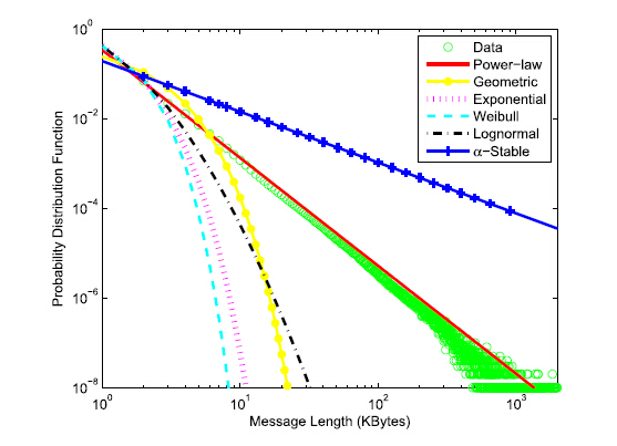
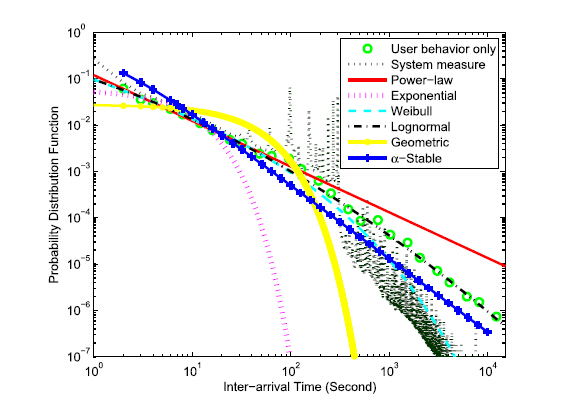
Compared with the geometric and exponential distribution functions recommended by 3GPP, power-law and lognormal distributions functions are more suitable to model the statistical pattern of message lengths and inter-arrival time of consecutive messages, respectively.

Due to their generality,  $\alpha$-Stable models are most suitable to characterize the aggregated traffic in cellular networks. Together with previous findings in fixed broadband networks, $\alpha$-Stable models are proven to accurately model the aggregated traffic from cellular access networks to core networks.

In addition, according to the generalized central limit theorem, the aggregated traffic within one BS, following  $\alpha$-Stable models, can be explained as the accumulation of a number of power-law distributed messages.

On the other hand, we have also investigated and characterized various kinds of traffic in wireless cellular networks, based on a large amount of real traffic data measurement. In particular, our dataset is based on a significant number of practical traffic records from one of the biggest cellular operators in an eastern provincial capital in China. The records in dataset are originated from nearly 10000 BSs with more than 10 million subscribers involved. Each traffic record has a resolution of 5 minutes, including timestamps, location area code (LAC), cell ID, application name and the corresponding volume of data traffic.

Concretely, IM(WeChat/Weixin), HTTP web browsing and QQLive Video are selected as the representatives of the three typical types of mobile service, IM, web browsing and video for discussion, respectively. Particularly, WeChat/Weixin is a widely booming social IM service which allows over 6 hundred million mobile users to exchange text messages and multimedia files like voices, pictures and videos with each other via smart phones, in China as well as around the world. The summary information on the mobile traffic dataset under study is listed in the following Table and Figures (e.g., Traffic time series of different mobile service types during one day).

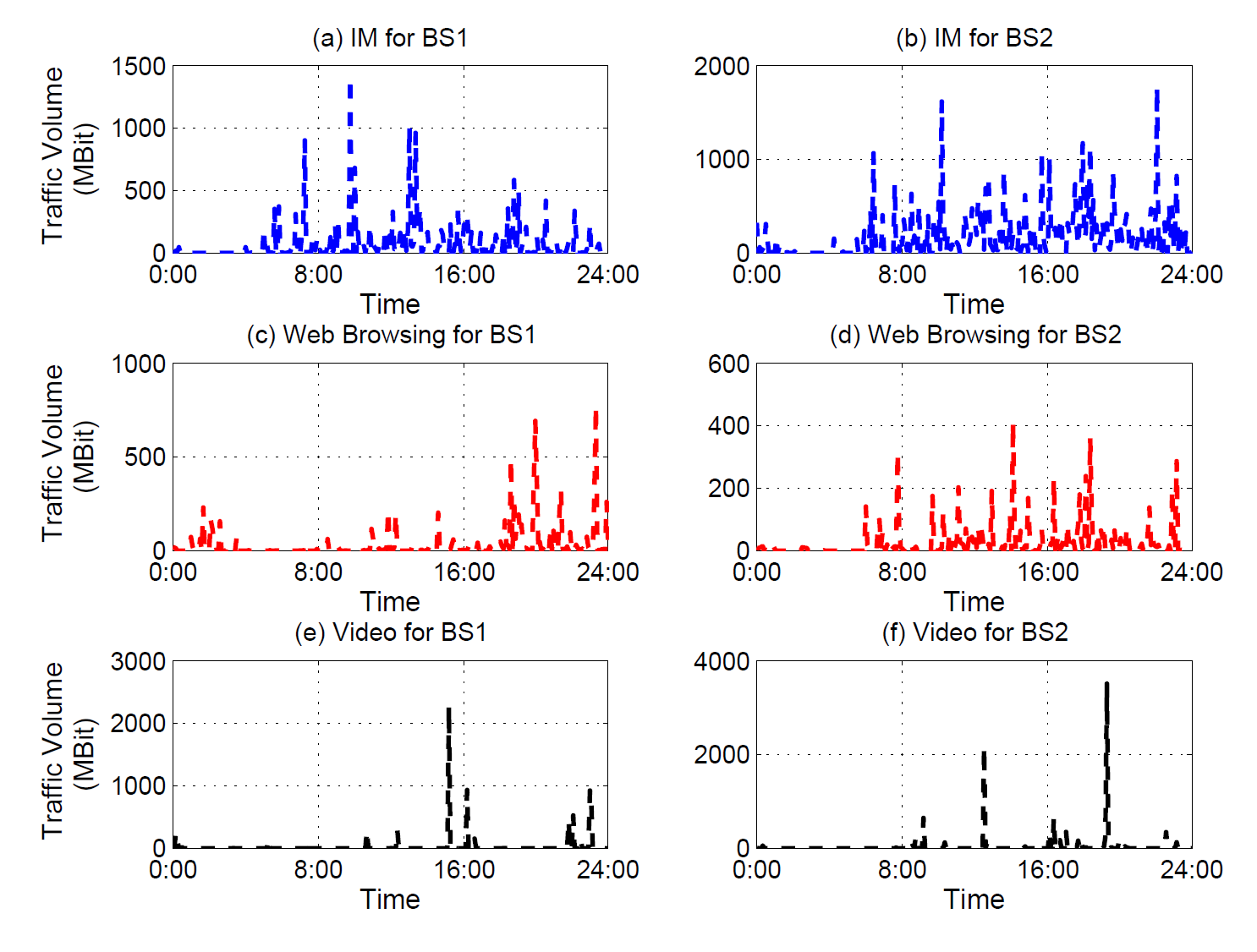
Remark 1. Application-level cellular data traffic series for IM, Web Browsing and video service appear bursty across a long range of time scales. The burstiness remains significant as the time scale increases.

Burst commonly implies sharp increase in volume of information interaction in seconds, which is potentially accompanied with the emergence of unexpected events or centralized activities of human beings. It is generally believed that bursty phenomena appears apparently and enormously in cellular data traffic series which is closely related to people’s daily life. In this section, we have a brief look at the burstiness of application-level cellular data traffic at different time scales and validate this intrinsic characteristics.

Remark 2. There widely exists self-similarity in application-level cellular data traffic in terms of   IM, Web browsing, and video services. Specifically, for IM and web browsing service, most traffic series exhibit a moderate degree of self-similarity while video service shows weaker self-similarity compared with the other two services under study.

In general, the parameter H is known as the Hurst parameter with the value ranging from 0.5 to 1.0 and has a positive correlation with the degree of self-similarity. That is to say, H =0.5 indicates the lack of self-similarity whereas large value for H (i.e., close to 1.0) indicates a large degree of self-similarity. Generally, graphical methods such as variance-time plot, R/S plot are used to test for self-similarity (see the following Figures).

Remark 3. According to the minor fitting errors, beside the MIM (WeChat/WeiXin), $\alpha$-Stable models are suitable to characterize all the other application-level data traffic in cellular networks.

In summary, we have demonstrated the universal existence of burstiness and self-similarity and their great significance in social mobile data traffic series. To capture these characteristics, $\alpha$-Stable distribution has been taken to model traffic series. The minor fitting errors for different service types verify the validity of $\alpha$-Stable models and the estimated parameter can reflect the characteristics of traffic series well.

---

Related references:

1. Rongpeng Li, Zhifeng Zhao, Chen Qi, Xuan Zhou, Yifan Zhou, and Honggang Zhang. “Understanding the Traffic Nature of Mobile Instantaneous Messaging in Cellular Networks: A Revisiting to $\alpha$-Stable Models,” IEEE Access, vol. 3, pp. 1416-1422, 2015.

2. Rongpeng Li, Zhifeng Zhao, Jianchao Zheng, Chengli Mei, Yueming Cai, and Honggang Zhang, “The Learning and Prediction of Application-level Traffic Data in Cellular Networks,” IEEE Trans. Wireless Communications, March 2017.

3. Zhifeng Zhao, Meng  Li, Rongpeng Li, and Yifan Zhou, “Temporal-Spatial Distribution Nature of Traffic and Base Stations in Cellular Networks,” IET Communications, August 2017.

4. Chen Qi, Zhifeng Zhao, Rongpeng Li, and Honggang Zhang, “Characterizing and Modeling Social Mobile Data Traffic in Cellular Networks,” 2016 IEEE 83rd Vehicular Technology Conference (VTC-Spring 2016), Nanjing, May 2016.

Dependence Between Base Stations Deployment and Traffic Spatial Distribution

Background

Base stations (BSs) deployment and traffic spatial distribution play crucial roles in network design and resource management. Actually, the BSs deployment and traffic spatial distribution are dually coupled, since BSs are built up to fulfill the traffic demand while data traffic is transmitted to mobile users through BSs. Thus it is imperative to fully understand BSs and traffic spatial distribution as well as statistical relationship between them.

Data Description

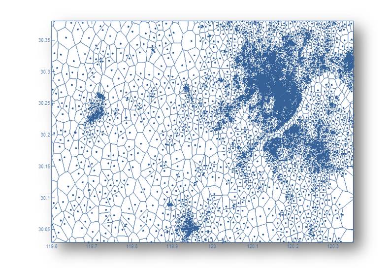
The data used in this paper is obtained from a commercial mobile operator in China. The dataset, collected from two kinds of networks (i.e., 2G and 3G cellular networks), includes traffic and BSs information. The data traffic is measured in the unit of bytes that each BS transmits to the covered users in one-hour interval. BSs information mainly involves geographic location (i.e., longitude, latitude, etc.) and BS type (i.e., macrocell or microcell).  Specifically, we convert the longitude and latitude values of each BS to X, Y coordinates, and plot the actual geographic location on an 2D coordinate plane as shown in Fig. 1 and Fig. 2.

Spatial Distribution of BSs and Traffic

Considering the real situations that heavy-tailed phenomenon does exist in BSs and traffic spatial distributions, we take $\alpha$-Stable distribution as the fitting candidate. The parameters of $\alpha$-Stable model are firstly estimated and the results are listed in Table II. Afterwards, we use the $\alpha$-Stable model, produced by the aforementioned estimated parameters, to generate some random variable, and compare the induced PDF with the exact (empirical) one. Therefore, as shown in Fig. 3 and Fig. 4, after fitting an $\alpha$-Stable distribution to BSs density and traffic spatial density in City A, they both better obey the $\alpha$-Stable distributions obviously. In City B, $\alpha$-Stable distribution is also applicable.

Linear Dependence Between BSs Density and Traffic Spatial Density

To ease illustration, Urban1 is taken as an representative example. With the sampling window size being 3x3 km^2^, 5x5 km^2^, 7x7 km^2^, then fitting results are depicted in Fig. 5. Evidently, BSs density and traffic spatial density exhibit strong linearity regardless of the BS type. Besides the visual observation, R- square value is also adopted as a performance metric to evaluate the goodness of fit. The closer is the value to 1, the better is the goodness of fit. According to Table III,  we find that linear regression model is reasonable to characterize the spatial correlation between BSs deployment and traffic spatial distribution, which can be stated as follows:

${\lambda }_{rmBS}=k{\lambda }_{rmTR}+t.$

Here, $k$ is a linear slope value that represents the needed number of BSs per unit spatial traffic.

On one hand, linear regression model keeps better fitting effect no matter the sample region is urban or rural. On the other hand, the key parameter slope k is closely associated with the BS type, without dependence on the sampling window size. These findings indicate that BSs deployment is deeply influenced by the subscribers’s demand as well as the corresponding traffic dynamics over the space, and imply that BSs density and traffic spatial density have almost identical heterogeneity feature.

Cellular Networks Evolution Trend

By comparing the fitted parameters in 2G and 3G scenes carefully, we discover that the $k_{2G,microcell}$ is greater than the $k_{2G,microcell}$  regardless of region type. The computed results are listed in Table IV. These experimental results demonstrate that an upgraded BS in 3G own more capacity and higher transmission rate than that in 2G.

Generally, some technological bottlenecks would be inevitable in cellular networks evolution for each generation.Therefore, new and advanced technologies have been explored to solve the confronted problems, thus achieving success in network upgrading and optimization. Particularly, in view of the difference of slope k in various cellular network scenarios, a reasonable assumption can be stated as follows:

$k_{2G}>k_{3G}>k_{4G}.$

In actual situations, however, with the increase of traffic load, it is impossible for the number of BSs to grow linearly and infinitely, due to the physical and performance constraints of each generation cellular network. Consequently, there should be a certain critical state for each generation cellular network. That is, the available service capability is pre-determined, and if traffic demand increases continuously, the network evolution would go through a network transition (i.e., upgrading from 2G to 3G, then to 4G). In that regard, an explanatory outline about how cellular network architecture evolves is illustrated in Fig. 6.

Whether it is a 2G era, 3G era or 4G era, linear dependence between BSs density and traffic spatial density always exists but with different slope k. Surely, the performance improvement of network expects BSs with larger capacity to supply more traffic demand meanwhile requires operators to implement less BSs to serve more subscribers in certain area.

Related references:

• Rongpeng Li, Zhifeng Zhao, Yi Zhong, Chen Qi, and Honggang Zhang, “The Stochastic Geometry Analyses of Cellular Networks with alpha-Stable Self-Similarity,” arxiv.org/abs/1709.05733v1, September 2017.

• Zhifeng Zhao, Meng  Li, Rongpeng Li, and Yifan Zhou, “Temporal-Spatial Distribution Nature of Traffic and Base Stations in Cellular Networks,” IET Communications, August 2017.

• Meng Li, Zhifeng Zhao, Yifan Zhou, Xianfu Chen, and Honggang Zhang, “On the Dependence Between Base Stations Deployment and Traffic Spatial Distribution in Cellular Networks,” 23rd International Conference on Telecommunications, Thessaloniki, Greece, May 2016.

 

The Emergence of Scaling Law, Fractal Patterns and Self-Similarity in Wireless Networks

Background

Cellular networks have been undergoing a long history of evolution and gradually accumulated unique spatial distribution pattern, as  BSs are continually deployed to provision the ever-increasing mobile traffic in hotspots accompanied by the global popularity of smart phones and tablets. Accordingly, by taking advantage of realistic traffic records from cellular networks, we can leverage the theory of complex networks to answer what is the intrinsic evolved nature in cellular networks? We first create a spatial traffic correlation model of BSs by regarding BSs as nodes and the traffic correlation between BSs as edges. Then, we analyze the structure and properties of this spatial traffic correlation model and derive the corresponding results in the networks. Interestingly, we discover that there exist three key properties, i.e., scale-free pattern, fractality, self-similarity, and small-world.

Data Acquisition and Preparation

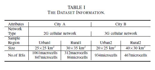
We acquire the real measurement data from one of the biggest commercial mobile operator in China, which contains the information of traffic and BSs from a second-generation (2G) cellular network in City A and the counterpart from a third-generation (3G) cellular network in City B. Specifically, the traffic data is measured in the unit of bytes that each BS transmits to the serving users. The related traffic for City A and City B lasts 7 days and 1 day, with one-hour and half-hour granularity, respectively. Therefore, for one BS, the traffic series for City A and City B could be regarded as a vector of 168 entries and 48 entries, respectively. Meanwhile, we plot the BS deployment with the geographical landforms in Fig. 1. Moreover, the BS related information such as BS type, location area and geographic location is available as well and more details are summarized in Table I.

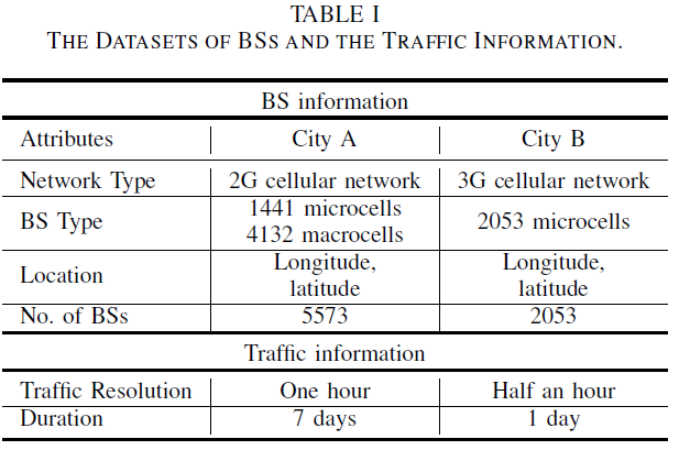
Fig. 1. An illustration of the deployment of base stations in two typical cities with geographical landforms, namely City A, B, respectively.

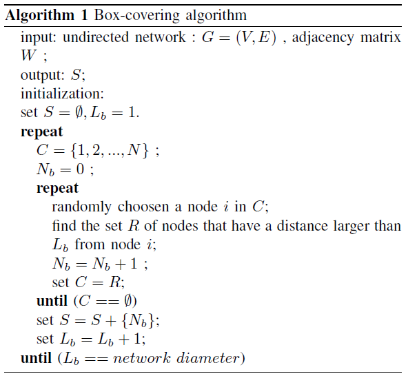
Box-covering Algorithm

As a widely used technique for characterizing fractal networks and calculating their fractal dimensions, box-covering algorithm has experienced a number of distinct versions since the generalized box-covering algorithm was introduced by Song . The random sequential (RS) box-covering algorithm  is not suitable in our work due to its low efficiency in finding the minimum number of boxes among all the possible tiling configurations. Therefore, we adopt a slightly improved algorithm  and detailed steps is shown in Algorithm. 1.

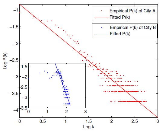
Analysis of Degree Distribution

Degree Distribution

The spatial traffic correlation model is built in terms of the traffic loads and contributes to understanding the underlying relationship of BSs, which can not be directly observed from brief information such as locations (e.g., longitude and latitude) or BS types. We provide the fitting results of the degree distributions of City A and City B. In general, the spatial traffic correlation model points to the property of scale-free and help us to know which BSs have higher degree values. The scale-free property from the traffic load correlation model clearly demonstrates that the minority of BSs with larger degree are highly correlated with plenty of other BSs, while the other remaining BSs are only correlated with a few number of BSs.

Identifying Influential Base Stations

Cellular networks have already employed macrocell BS as the signaling node, so the macrocell BSs are more suitable to be influential nodes due to their greater coverage capability and being more easily to predict the tendency of BS traffic loads. As a result, it is imperative to pick out the most important BSs so as to assign them more functions such as signaling control. Based on the theory of influence maximization in complex networks, we further employ the CI algorithm for localizing the most influential BSs.

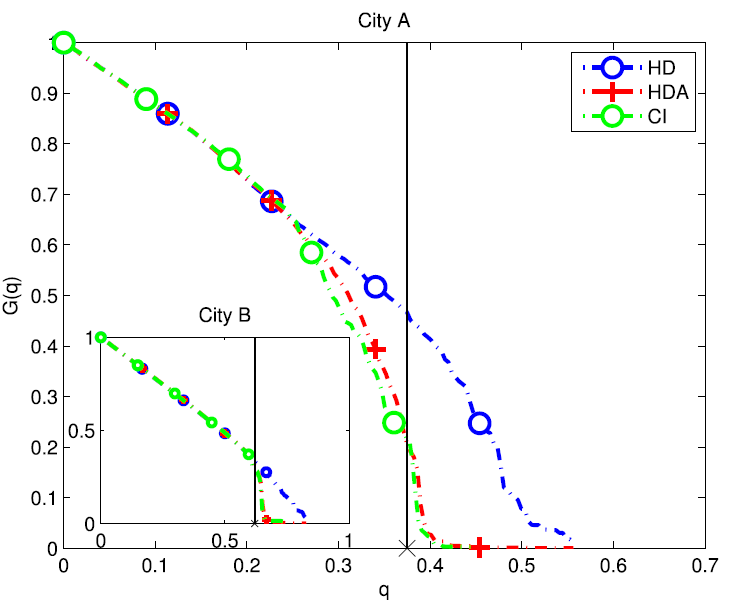
Fig. 3. Performance of CI in correlation model compared with heuristic methods (HD, HDA).

Afterwards, according to the optimal set of nodes found by the CI algorithm, we display the locations of the most influential 500 base stations of City A in the map and color codes each BS’s degree in Fig. 4 and Fig. 5. From the two figures, we observe that among the most influential base stations extracted by the CI algorithm, a large number of low-degree BSs even exhibit a greater influence than some high-degree BSs. That is to say, we should pay more attention to those influential BSs even with low-degree, comparing with the high-degree BSs with less influence.

Structural Properties of the Traffic Load Correlation Model

Fractal Patterns

One important property that exists in many complex and real-world networks is fractality. In fractal geometry, box-covering is widely used to approximately evaluate the fractal dimension of a fractal object.

Fig. 6. Fractal patterns of City A and City B with the same threshold K 0.54.

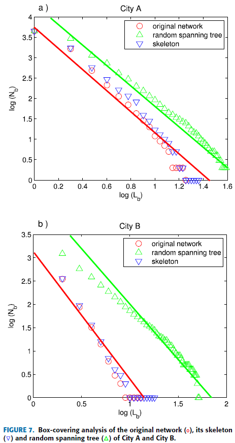
Skeleton Features

Basically, skeleton is thought to be a maximum spanning tree. Thus, the skeleton of our correlated BSs network is a spanning tree connected by the most close links, whose topology can be regarded as the core of the correlated BSs network.

After tiling the skeletons with the box-covering algorithm, the number of boxes needed to cover the networks is almost identical with the original networks. The box-covering analysis results of the original network, the skeleton and the random spanning tree are provided in Fig. 7. According to the curves, the relevant results express that although the random spanning tree possesses a different statistics, the fractal dimensions of the random spanning tree and the original network are just the same. Meanwhile, the fractality of the skeleton matches the fractality of the original correlation model very well. Hence, understanding the properties of the skeleton is of great importance for analyzing the original model.

Further Exploration On Small-World

The small-world property usually coexists with scale-free networks. Specically, small-world property refers to the average distance d scales logarithmically with the network size N . Another indispensable characteristic of small-world networks is their high clustering coeffcient.

We have demonstrated that the spatial traffic correlation model of BSs expresses scale-free, fractal and small-world properties simultaneously, which will further facilitate the performance analysis of complex cellular networks as well as the design of efficient networking protocols. Moreover, for a topological structure with fractality, we can  find some regularities from its special topology and irregularity, which contributes to more effective resource assignment based on dynamic BSs management. Finally, the discovery of small-world property means that, despite the large-scale feature of the traffic load correlation model, the traffic association on base stations is very compact.

---

Related references:

• Chao Yuan, Zhifeng Zhao, Rongpeng Li, M. Li, and Honggang Zhang, “The Emergence of Scaling Law, Fractal Patterns and Small-World in Wireless Networks,” IEEE Access, March 2017.

• Rongpeng Li, Zhifeng Zhao, Yi Zhong, Chen Qi, and Honggang Zhang, “The Stochastic Geometry Analyses of Cellular Networks with α-Stable Self-Similarity,” IEEE Trans. on Communications, March 2019.

• Ying Chen, Rongpeng Li, Zhifeng Zhao, and Honggang Zhang, “Study on Base Station Topology in National Cellular Networks: Take Advantage of Alpha Shapes, Betti Numbers, and Euler Characteristics,” IEEE Systems Journal, Q3/Q4 2019.

• Ying Chen, Rongpeng Li, Zhifeng Zhao, and Honggang Zhang, “Fundamentals on Base Stations in Urban Cellular Networks: From the Perspective of Algebraic Topology,” IEEE Wireless Communications Letters, April 2019.

• Rongpeng Li, Zhifeng Zhao, Yi Zhong, Chen Qi, and Honggang Zhang, “The Stochastic Geometry Analyses of Cellular Networks with alpha-Stable Self-Similarity,” arxiv.org/abs/1709.05733v1, September 2017.

• Ying Chen, Rongpeng Li, Zhifeng Zhao, and Honggang Zhang, “On the Capacity of Wireless Networks With Fractal and Hierarchical Social Communications,” arxiv.org/abs/1708.04585, August 2017.

• Ying Chen, Rongpeng Li, Zhifeng Zhao, and Honggang Zhang, “On the Capacity of Fractal Wireless Networks With Direct Social Interactions,” arXiv:1705.09751, May 27, 2017.

• Rongpeng Li, Zhifeng Zhao, Jianchao Zheng, Chengli Mei, Yueming Cai, and Honggang Zhang, “The Learning and Prediction of Application-level Traffic Data in Cellular Networks,” IEEE Trans. Wireless Communications, March 2017.

• Zhifeng Zhao, Meng  Li, Rongpeng Li, and Yifan Zhou, “Temporal-Spatial Distribution Nature of Traffic and Base Stations in Cellular Networks,” IET Communications, August 2017.

• Chen Qi, Zhifeng Zhao, Rongpeng Li, and Honggang Zhang, “Characterizing and Modeling Social Mobile Data Traffic in Cellular Networks,” 2016 IEEE 83rd Vehicular Technology Conference (VTC-Spring 2016), Nanjing, May 2016.